MLP vs KAN on a Real Graph Task
This page shares my MLP results on the same dataset used in my KAN write-up, and then briefly compares the two. For the KAN post, see the full KAN article. See the GitHub repo for code and data: GitHub - SSareen/food-network-analysis-kan.
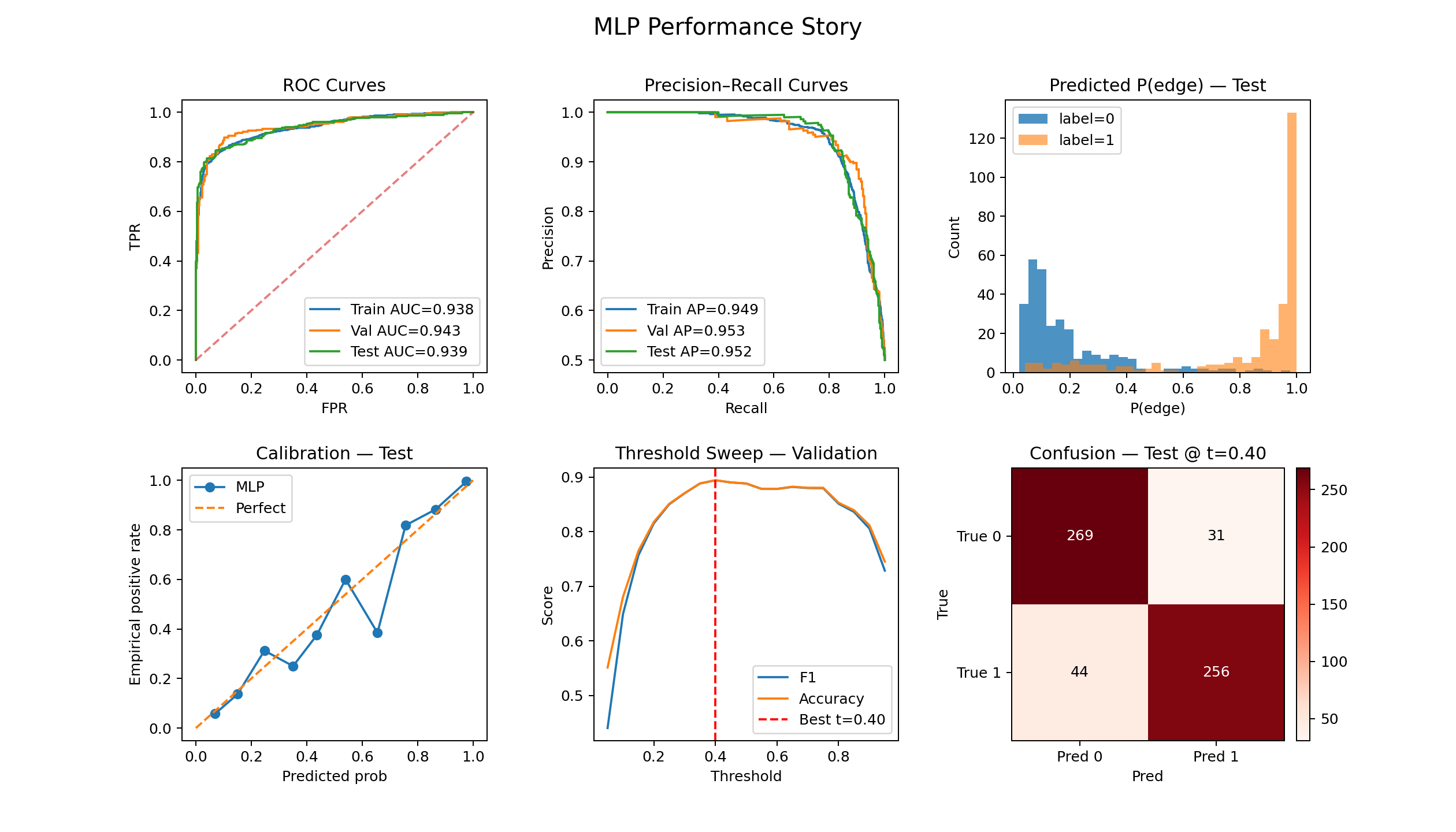
Results at a Glance
- Both models perform similarly: ROC-AUC ≈ 0.93, Accuracy/F1 ≈ 0.88.
- Decision threshold matters: MLP’s best validation threshold ≈ 0.40 (not 0.5); KAN’s best ≈ 0.26.
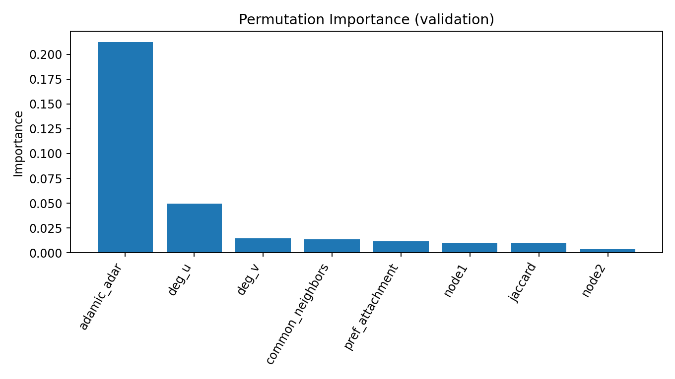
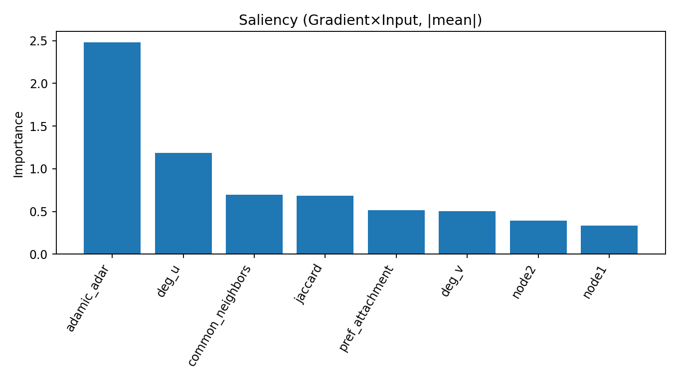
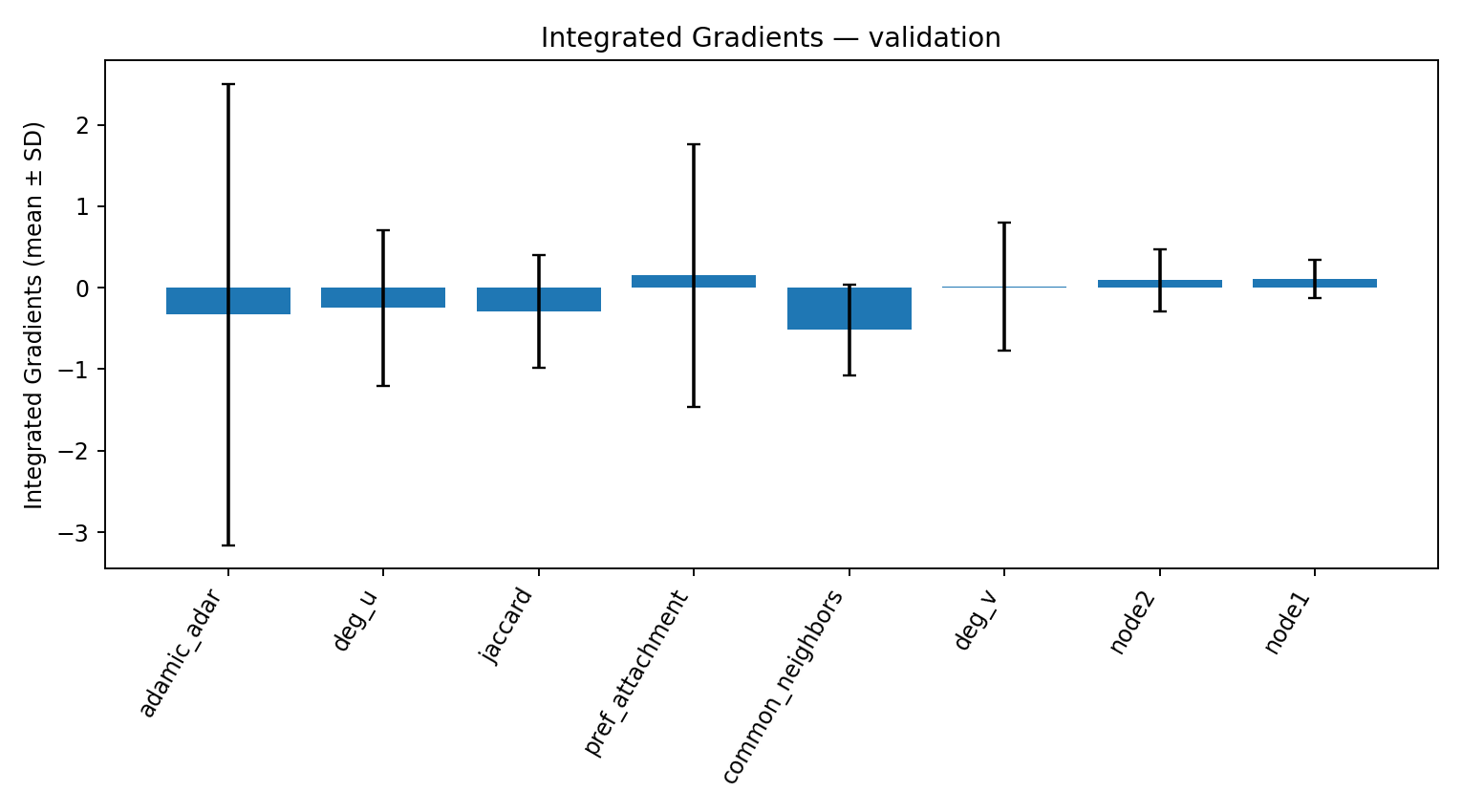
- Top signal agrees: both rank Adamic-Adar as the most informative feature.
- Runner-up differs: KAN elevates common_neighbors #2; MLP elevates deg_u #2 (see below sections).
Comparison to KANs
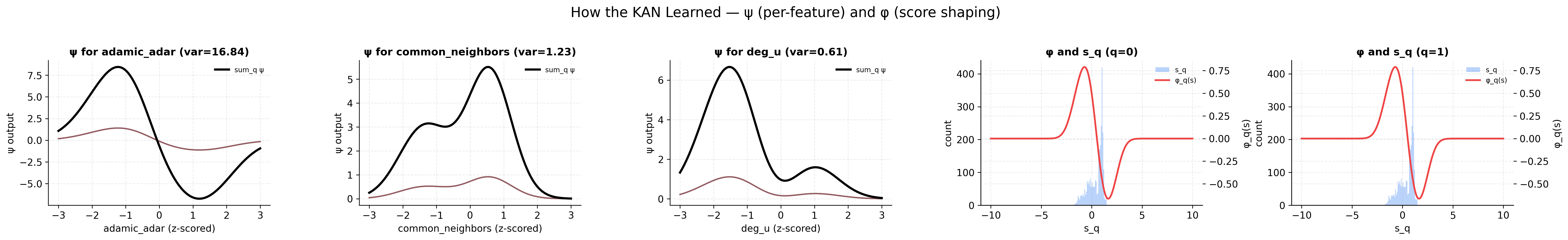
On this dataset, MLP and KAN land in the same performance band. The difference is in how much they tell us about why they work: KAN exposes feature-shape curves (ψ/φ) that show where each feature helps most (including non-monotonic “sweet spots”), while the MLP requires attribution tools to infer that behavior. Both agree that Adamic-Adar is #1; they diverge on #2.
Why KAN ranks Common Neighbors #2 but MLP ranks deg(u) #2
KAN learns a curve for Common Neighbors (CN) directly, so it can decide that “a medium amount of shared neighbors is most useful; very low or very high CN helps less.” MLP doesn’t show that curve explicitly. Instead, it uses the degree of node u as a context knob to judge whether a given CN is meaningful. In other words, the same CN value means different things for a small page vs. a hub, so degree(u) ends up highly useful in the MLP’s attributions.
- Pair A: CN = 5, deg(u) = 18 (small page) → 5 shared neighbors is strong evidence of a link.
- Pair B: CN = 5, deg(u) = 800 (hub) → 5 shared neighbors is weak; hubs share neighbors with many pages.
Bottom line: KAN gives more credit to CN because it models the usefulness of CN itself (with a learned shape). The MLP gives more credit to degree(u) because it needs degree to interpret whether a CN count is informative or just hub noise.
Glossary
Permutation importance. Shuffle one feature’s values and re-score the model; the drop in a metric (e.g., AUC) estimates that feature’s global usefulness.
Saliency (|grad×input|). Measures how sensitive the prediction is to tiny nudges in a feature around each data point; bigger values mean stronger local influence.
Integrated Gradients. Measures a feature’s contribution by summing the model’s response as that feature goes from a baseline (e.g., zero) to its actual value; larger magnitude = more influence, sign (+/−) = direction.
Dataset citation:
@inproceedings{nr,
    title={The Network Data Repository with Interactive Graph Analytics and Visualization},
    author={Ryan A. Rossi and Nesreen K. Ahmed},
    booktitle={AAAI},
    url={https://networkrepository.com},
    year={2015}
}