Introduction to Kolmogorov–Arnold Networks

Introduction to Kolmogorov-Arnold Networks

Simran Sareen | July 19, 2025

Every continuous function of several variables can be built from simple one‑dimensional curves and addition. In 1957, Kolmogorov and Arnold proved that any multivariate function

$$ f(x_{1},\dots,x_{n}) $$

admits the form

$$ f(x) = \sum_{q=1}^{2n+1} \Phi_{q}\left(\sum_{p=1}^{n}\phi_{q,p}(x_{p})\right) $$

where each $\phi_{q,p}$ and $\Phi_{q}$ is a function of a single real variable. All mixing happens by sums; each bend is only ever one‑dimensional.

1. A Tiny Worked Example

Take the simplest case, two inputs $(x,y)$ and

$$ f(x,y) = x + y $$

Here $n = 2$, so we have up to $2 \cdot 2 + 1 = 5$ terms of the form $\Phi_{q}(\phi_{q,1}(x)+\phi_{q,2}(y))$. We set:

Term 1: $\phi_{1,1}(x)=x$, $\phi_{1,2}(y)=0$, $\Phi_{1}(u)=u$ → $x$
Term 2: $\phi_{2,1}(x)=0$, $\phi_{2,2}(y)=y$, $\Phi_{2}(u)=u$ → $y$
Terms 3-5: all-zero maps → $0$

Summing them recovers $x + y$. The extra slots simply stay inactive.

2. From Theorem to Network

We turn that formula into a two‑layer network:

Input layer: One node per coordinate $x_{p}$.
First layer of edges: Connection $p\to q$ applies the univariate function $\phi_{q,p}$ to $x_{p}$.
Hidden nodes: Node $q$ sums its incoming values: $s_{q} = \sum_{p=1}^{n} \phi_{q,p}(x_{p})$.
Second layer of edges: Connection $q\to$ output applies $\Phi_{q}$ to $s_{q}$.
Output node: Sums all $\Phi_{q}(s_{q})$ to produce $f(x)$.

No activation at nodes; every non‑linearity lives on edges.

3. Anatomy of a 2‑D KAN Layer

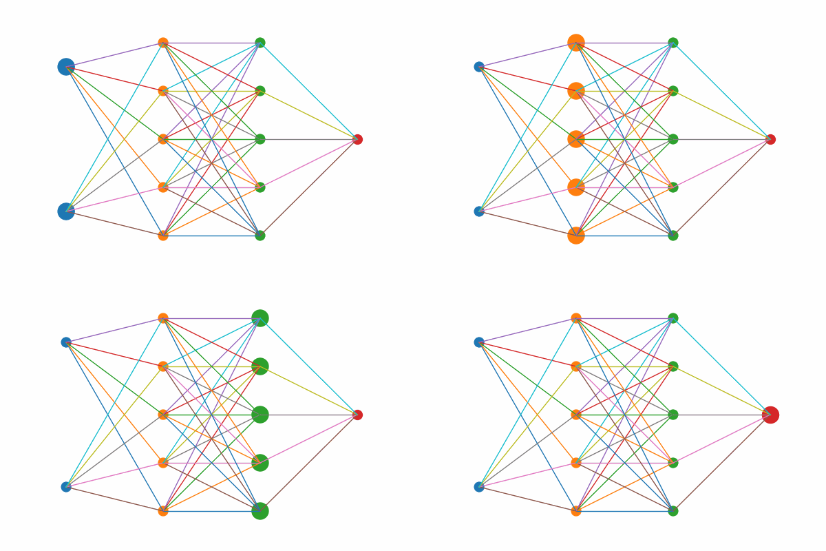
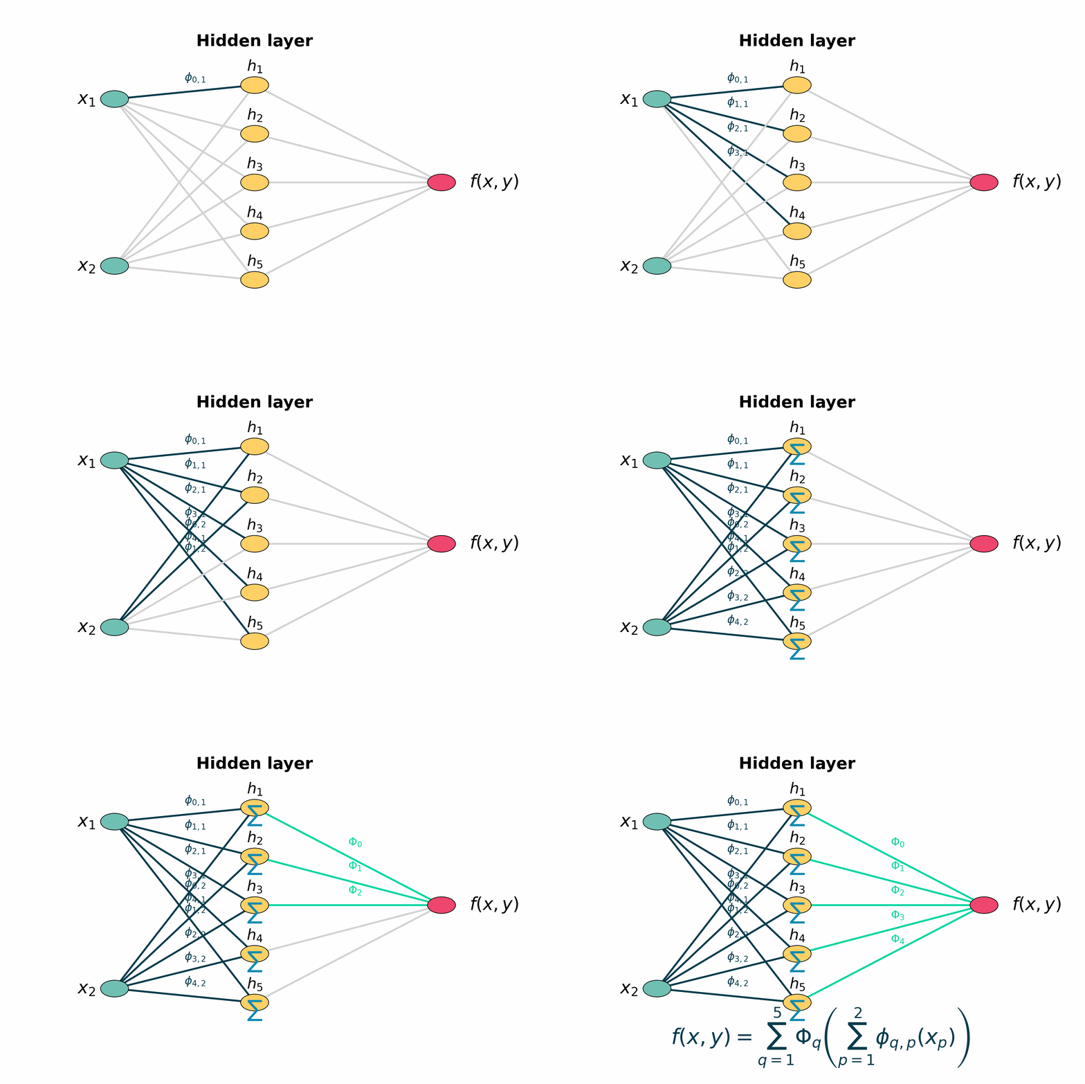
For $n=2$, the hidden layer has $2\cdot2+1=5$ summing nodes. Each wire is its own $\phi$ or $\Phi$, and each hidden node just adds.

Figure 1: Layer by layer animation of KAN structure

Figure 1: Layers highlights first the two input nodes, then the five hidden sums, then the five output‐mapping edges, and finally the output node. KAN colored animated GIF

Figure 2: Animated edge-wise functional activations

Figure 2: Shows all connections in sequence. Each edge carries its own independent activation function.

4. The Layer as a Matrix of Functions

A KAN layer isn’t weights times inputs. It’s a matrix whose entries are functions. If layer $l$ has $n_{l}$ inputs and $n_{l+1}$ outputs, then:

$$ \mathbf{x}_{l+1} = \begin{pmatrix} \phi_{l,1,1}(x_{l,1}) & \phi_{l,1,2}(x_{l,2}) & \dots & \phi_{l,1,n_{l}}(x_{l,n_{l}})\\ \phi_{l,2,1}(x_{l,1}) & \phi_{l,2,2}(x_{l,2}) & \dots & \phi_{l,2,n_{l}}(x_{l,n_{l}})\\ \vdots & \vdots & \ddots & \vdots\\ \phi_{l,n_{l+1},1}(x_{l,1}) & \phi_{l,n_{l+1},2}(x_{l,2}) & \dots & \phi_{l,n_{l+1},n_{l}}(x_{l,n_{l}}) \end{pmatrix} $$

To get each $x_{l+1,j}$, apply that row’s functions to the input coordinates and sum:

$$ x_{l+1,j} = \sum_{i=1}^{n_{l}} \phi_{l,j,i}(x_{l,i}) $$

5. Building Edge Activations with B‑Splines

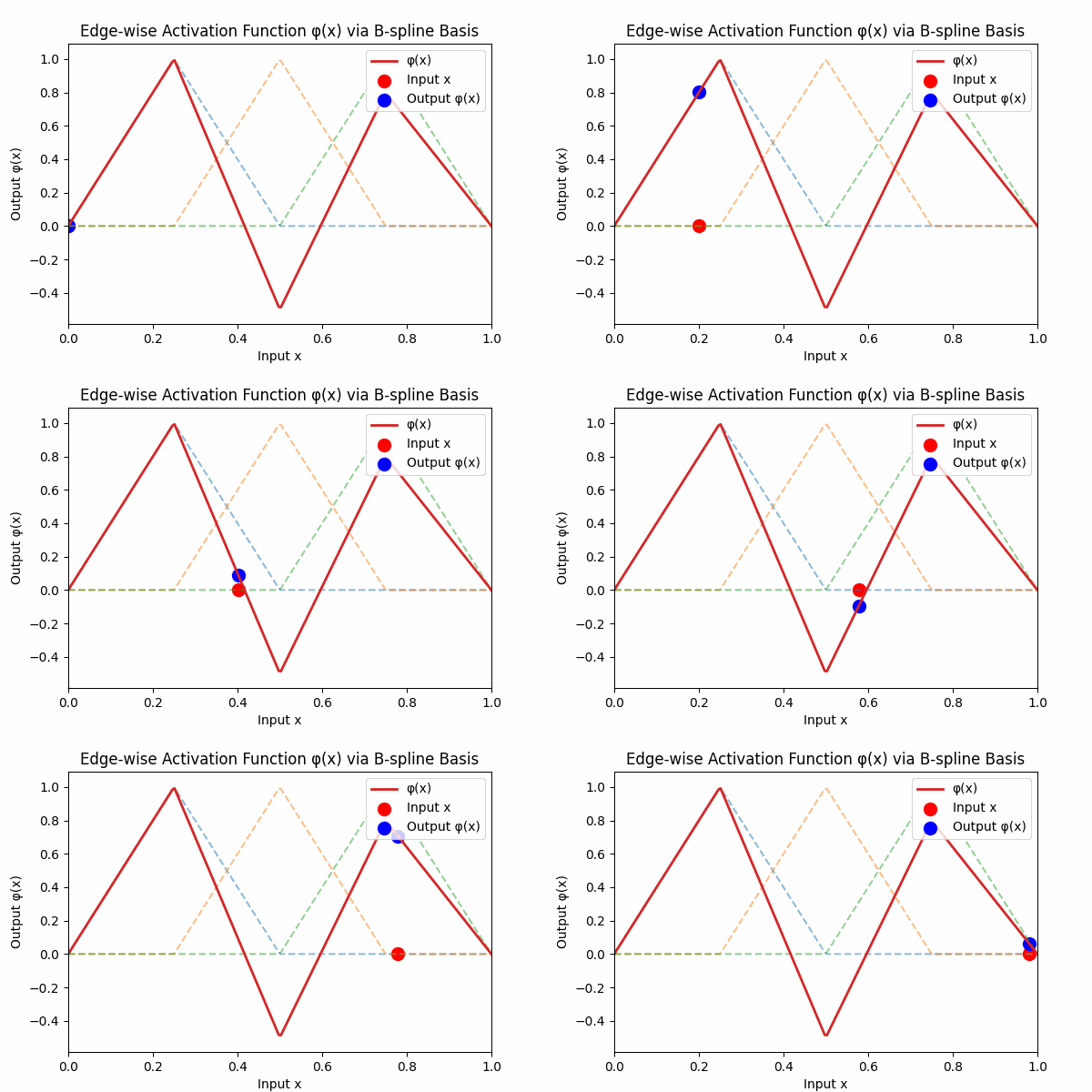
Each edge activation $\phi(x)$ is a smooth curve built from simple basis hats:

Figure 3: Weighted B-spline sum to form activation curve

Figure 3: The dashed lines are individual B‑spline basis functions $ B_k(x) $. The thick red curve is their weighted sum $ \phi(x) = \sum_k w_k B_k(x) $. Each basis vanishes outside its knot interval, so $ \phi $ returns to zero at the boundaries.

6. How KANs Differ from MLPs

Aspect	Standard MLP	KAN Network
Edges	Carry scalar weights	Carry full functions ($\phi, \Phi$)
Nodes	Sum then activate	Sum only; no node activations
Non-linearity	Lives at nodes	Lives on edges (purely one-dimensional)
Mixing vs Bending	Edges mix, nodes bend	Edges bend, nodes mix

7. Going Deeper

A basic KAN has shape $[n, 2n+1, 1]$. To add depth, insert any number of intermediate layers of size $2n+1$:

$$ [n, 2n+1, 2n+1, \dots, 2n+1, 1] $$

8. Common Confusions

Why $2n+1$ hidden nodes?
That exact width is what the theorem guarantees. Fewer nodes can’t capture every possible interaction among the $n$ inputs; extra terms simply stay zero for simple functions.
Pre-activation vs Post-activation
- Pre-activation $x_{l,i}$: the raw number at node $(l,i)$.
- Post-activation $\phi_{l+1,j,i}(x_{l,i})$: that number after its edge-wise bend en route to node $(l+1,j)$.
Matrix-of-Functions view
Each layer’s matrix entry $\phi_{l,j,i}(\cdot)$ is the curve on edge $i\to j$. Computing the next layer means applying each curve to its input coordinate and summing along each row.

9. End-to-End Process: MLP vs KAN

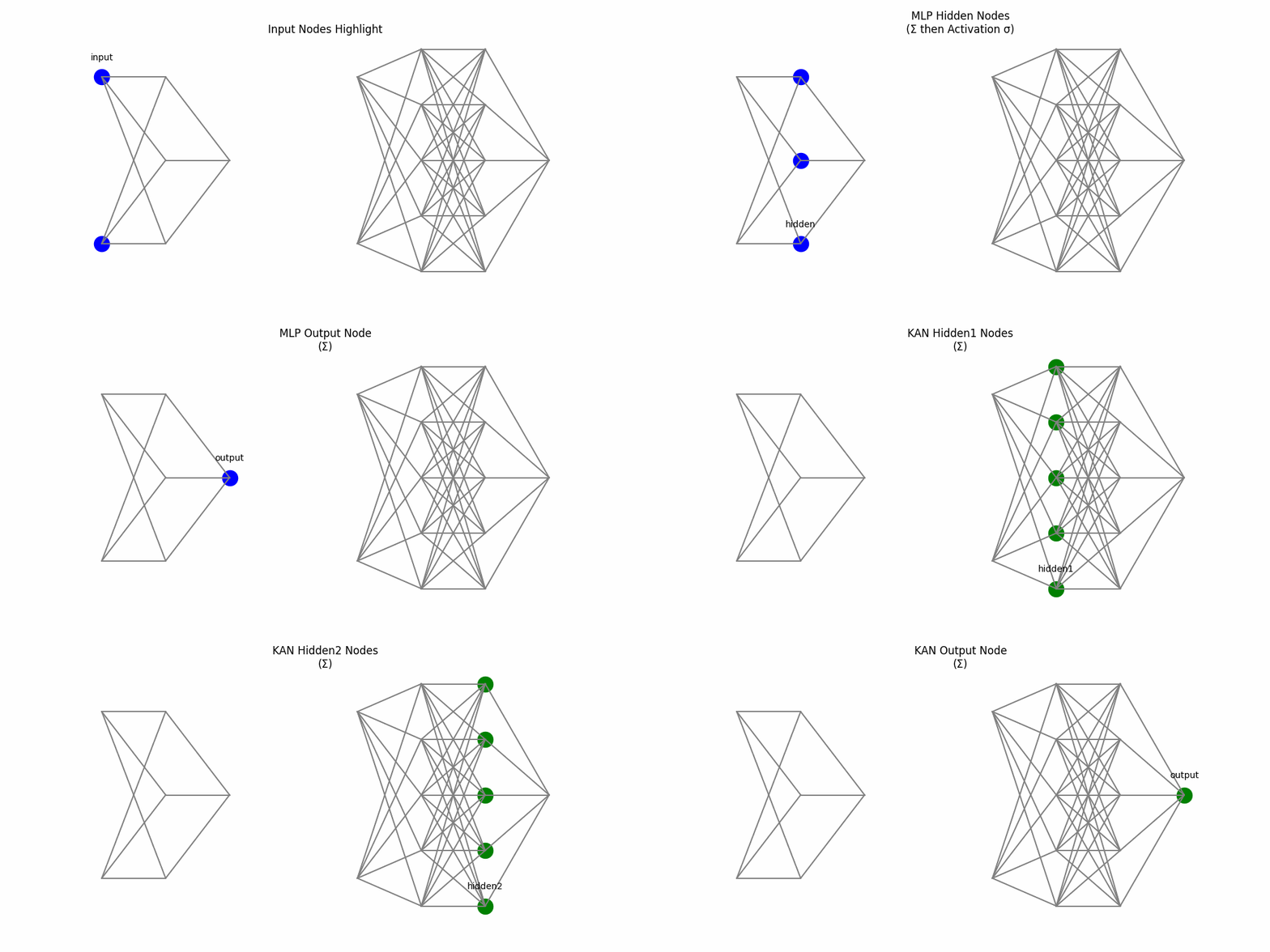
Here’s a side-by-side animation comparing a two-layer MLP (left) and a two-layer KAN (right):

Figure 4: Side-by-side: MLP weights and node activations vs KAN edge activations and summing nodes

1. Inputs activate.
2. MLP edges multiply by weights; KAN edges apply univariate functions.
3. MLP hidden nodes sum then activate; KAN hidden nodes sum only.
4. Edges to output carry weights vs edge-wise activations.
5. Final summation produces the output.

Aspect	Standard MLP	KAN Network
Edges	Carry scalar weights	Carry full functions (\(\phi, \Phi\))
Nodes	Sum then activate	Sum only; no node activations
Non-linearity	Lives at nodes	Lives on edges (purely one-dimensional)
Mixing vs Bending	Edges mix, nodes bend	Edges bend, nodes mix